Conditional expressions CASE. CASE conditional expressions CASE expression is a conditional statement of the SQL language
CASE expression
DECODE function
Two methods are used:
The two methods that are used to implement conditional processing (IF-THEN-ELSE logic) in an SQL statement are the CASE expression and the DECODE function.
Note: The CASE expression conforms to ANSI SQL. The DECODE function is specific to the Oracle syntax.
CASE expression
Simplifies conditional queries by making the IF-THEN-ELSE statement work:
CASE expressions allow you to use IF-THEN-ELSE logic in SQL statements without having to call procedures.
In simple conditional expression CASE Oracle Server searches for the first WHEN ... THEN pair for which expr equals comparison_expr and returns return_expr. If none of the WHEN ... THEN pairs satisfy this condition, and if the else clause exists, Oracle returns else_expr. Otherwise, Oracle returns null. You cannot specify NULL for all return_exprs and else_expr.
Expr and comparison_expr must be the same data type, which can be CHAR, VARCHAR2, NCHAR, or NVARCHAR2. All return values (return_expr) must be of the same data type.
In this syntax, Oracle compares the input expression (e) to each comparison expression e1, e2, ..., en.
If the input expression equals any comparison expression, the CASE expression returns the corresponding result expression (r).
If the input expression e does not match any comparison expression, the CASE expression returns the expression in the ELSE clause if the ELSE clause exists, otherwise, it returns a null value.
Oracle uses short-circuit evaluation for the simple CASE expression. It means that Oracle evaluates each comparison expression (e1, e2, .. en) only before comparing one of them with the input expression (e). Oracle does not evaluate all comparison expressions before comparing any of them with the expression (e). As a result, Oracle never evaluates a comparison expression if a previous one equals the input expression (e).
Simple CASE expression example
We will use the products table in the for the demonstration.
The following query uses the CASE expression to calculate the discount for each product category i.e., CPU 5%, video card 10%, and other product categories 8%
SELECT CASE category_id WHEN 1 THEN ROUND (list_price * 0.05,2) - CPU WHEN 2 THEN ROUND (List_price * 0.1,2) - Video Card ELSE ROUND (list_price * 0.08,2) - other categories END discount FROM ORDER BY |
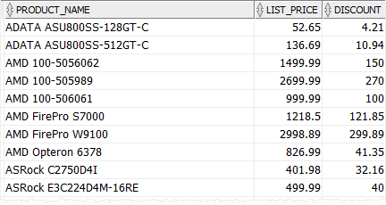
Note that we used the ROUND () function to round the discount to two decimal places.
Searched CASE expression
The Oracle searched CASE expression evaluates a list of Boolean expressions to determine the result.
The searched CASE statement has the following syntax:
CASE WHEN e1THEN r1 , COUNT (DISTINCT DepartmentID) [Number of Unique Departments], COUNT (DISTINCT PositionID) [Number of Unique Positions], COUNT (BonusPercent) [Number of Employees with% Bonus], MAX (BonusPercent) [Maximum Bonus Percentage], MIN (BonusPercent) [Minimum bonus percentage], SUM (Salary / 100 * BonusPercent) [Sum of all bonuses], AVG (Salary / 100 * BonusPercent) [Average bonus], AVG (Salary) [Average salary] FROM Employees Let's take a look at how each return value came about, and in one go, let's recall the constructions of the basic syntax of the SELECT statement. First, because we did not specify WHERE conditions in the query, then the totals will be calculated for the detailed data that is obtained by the query: SELECT * FROM Employees Those. for all rows of the Employees table. For clarity, we will select only the fields and expressions that are used in aggregate functions: SELECT DepartmentID, PositionID, BonusPercent, Salary / 100 * BonusPercent, Salary FROM Employees
This is the initial data (detailed lines) by which the totals of the aggregated query will be calculated. Now let's take a look at each aggregated value:
Let's summarize some of the results:
Accordingly, when setting an additional condition with aggregate functions in the WHERE clause, only totals will be calculated for rows that satisfy the condition. Those. the calculation of aggregate values is performed for the total set, which is obtained using the SELECT construction. For example, let's do everything the same, but only in the context of the IT department: SELECT COUNT (*) [Total number of employees], COUNT (DISTINCT DepartmentID) [Number of unique departments], COUNT (DISTINCT PositionID) [Number of unique positions], COUNT (BonusPercent) [Number of employees with% bonus] , MAX (BonusPercent) [Maximum bonus percentage], MIN (BonusPercent) [Minimum bonus percentage], SUM (Salary / 100 * BonusPercent) [Sum of all bonuses], AVG (Salary / 100 * BonusPercent) [Average bonus size], AVG (Salary) [Average Salary] FROM Employees WHERE DepartmentID = 3 - Consider only IT department SELECT DepartmentID, PositionID, BonusPercent, Salary / 100 * BonusPercent, Salary FROM Employees WHERE DepartmentID = 3 - only include IT department
Go ahead. If the aggregate function returns NULL (for example, all employees do not have the Salary value), or not a single record was included in the selection, and in the report, for such a case we need to show 0, then the ISNULL function can wrap the aggregate expression: SELECT SUM (Salary), AVG (Salary), - process the total using ISNULL ISNULL (SUM (Salary), 0), ISNULL (AVG (Salary), 0) FROM Employees WHERE DepartmentID = 10 - a non-existent department is specially indicated here to prevent the query from returning records
I believe that it is very important to understand the purpose of each aggregate function and how they calculate it, because in SQL, it is the main tool for calculating totals. In this case, we examined how each aggregate function behaves independently, i.e. it was applied to the values of the entire recordset obtained by the SELECT command. Next, we'll look at how these same functions are used to calculate group totals using the GROUP BY clause. GROUP BY - grouping dataBefore that, we have already calculated totals for a specific department, roughly as follows:SELECT COUNT (DISTINCT PositionID) PositionCount, COUNT (*) EmplCount, SUM (Salary) SalaryAmount FROM Employees WHERE DepartmentID = 3 - data for IT department only Now imagine that we were asked to get the same figures for each department. Of course, we can roll up our sleeves and fulfill the same request for each department. So, no sooner said than done, we write 4 requests: SELECT "Administration" Info, COUNT (DISTINCT PositionID) PositionCount, COUNT (*) EmplCount, SUM (Salary) SalaryAmount FROM Employees WHERE DepartmentID = 1 - data on Administration SELECT "Accounting" Info, COUNT (DISTINCT PositionID) PositionCount, COUNT ( *) EmplCount, SUM (Salary) SalaryAmount FROM Employees WHERE DepartmentID = 2 - Accounting data SELECT "IT" Info, COUNT (DISTINCT PositionID) PositionCount, COUNT (*) EmplCount, SUM (Salary) SalaryAmount FROM Employees WHERE DepartmentID = 3 - data on IT department SELECT "Other" Info, COUNT (DISTINCT PositionID) PositionCount, COUNT (*) EmplCount, SUM (Salary) SalaryAmount FROM Employees WHERE DepartmentID IS NULL - and don't forget data on freelancers As a result, we get 4 datasets:
Please note that we can use fields specified as constants - "Administration", "Accounting", ... In general, we extracted all the numbers that were asked of us, we combine everything in Excel and give it to the director. The director liked the report, and he says: "and add another column with information on the average salary." And as always, it needs to be done very urgently. Hmm, what to do ?! In addition, let's imagine that our departments are not 3, but 15. This is exactly what the GROUP BY clause is for such cases: SELECT DepartmentID, COUNT (DISTINCT PositionID) PositionCount, COUNT (*) EmplCount, SUM (Salary) SalaryAmount, AVG (Salary) SalaryAvg - plus we fulfill the wishes of the director FROM Employees GROUP BY DepartmentID
We got all the same data, but now using only one request! For now, do not pay attention to the fact that our departments are displayed in the form of numbers, then we will learn how to display everything beautifully. In the GROUP BY clause, you can specify several fields "GROUP BY field1, field2, ..., fieldN", in this case the grouping will occur by groups that form the values of these fields "field1, field2, ..., fieldN". For example, let's group the data by Departments and Positions: SELECT DepartmentID, PositionID, COUNT (*) EmplCount, SUM (Salary) SalaryAmount FROM Employees GROUP BY DepartmentID, PositionID SELECT COUNT (*) EmplCount, SUM (Salary) SalaryAmount FROM Employees WHERE DepartmentID IS NULL AND PositionID IS NULL SELECT COUNT (*) EmplCount, SUM (Salary) SalaryAmount FROM Employees WHERE DepartmentID = 1 AND PositionID = 2 - ... SELECT COUNT (*) EmplCount, SUM (Salary) SalaryAmount FROM Employees WHERE DepartmentID = 3 AND PositionID = 4 And then all these results are combined together and given to us as one set:
From the main one, it is worth noting that in the case of grouping (GROUP BY), in the list of columns in the SELECT block:
And a demonstration of all that was said: SELECT "String constant" Const1, - constant in the form of string 1 Const2, - constant in the form of a number - expression using the fields participating in the group CONCAT ("Department No.", DepartmentID) ConstAndGroupField, CONCAT ("Department No.", DepartmentID , ", Position No.", PositionID) ConstAndGroupFields, DepartmentID, - field from the list of fields participating in the grouping - PositionID, - the field participating in the grouping, it is not necessary to duplicate here COUNT (*) EmplCount, - number of lines in each group - the rest of the fields can only be used with aggregate functions: COUNT, SUM, MIN, MAX,… SUM (Salary) SalaryAmount, MIN (ID) MinID FROM Employees GROUP BY DepartmentID, PositionID - grouping by fields DepartmentID, PositionID It is also worth noting that grouping can be done not only by fields, but also by expressions. For example, let's group the data by employees, by year of birth: SELECT CONCAT ("Year of birth -", YEAR (Birthday)) YearOfBirthday, COUNT (*) EmplCount FROM Employees GROUP BY YEAR (Birthday) Let's look at an example with a more complex expression. For example, let's get the gradation of employees by year of birth: SELECT CASE WHEN YEAR (Birthday)> = 2000 THEN "from 2000" WHEN YEAR (Birthday)> = 1990 THEN "1999-1990" WHEN YEAR (Birthday)> = 1980 THEN "1989-1980" WHEN YEAR (Birthday)> = 1970 THEN "1979-1970" WHEN Birthday IS NOT NULL THEN "before 1970" ELSE "not specified" END RangeName, COUNT (*) EmplCount FROM Employees GROUP BY CASE WHEN YEAR (Birthday)> = 2000 THEN "from 2000" WHEN YEAR (Birthday)> = 1990 THEN "1999-1990" WHEN YEAR (Birthday)> = 1980 THEN "1989-1980" WHEN YEAR (Birthday)> = 1970 THEN "1979-1970" WHEN Birthday IS NOT NULL THEN "before 1970" ELSE "not specified" END
Those. in this case, the grouping is done according to the CASE-expression previously calculated for each employee: SELECT ID, CASE WHEN YEAR (Birthday)> = 2000 THEN "from 2000" WHEN YEAR (Birthday)> = 1990 THEN "1999-1990" WHEN YEAR (Birthday)> = 1980 THEN "1989-1980" WHEN YEAR (Birthday) > = 1970 THEN "1979-1970" WHEN Birthday IS NOT NULL THEN "before 1970" ELSE "not specified" END FROM Employees
And of course, you can combine expressions with fields in the GROUP BY block: SELECT DepartmentID, CONCAT ("Year of birth -", YEAR (Birthday)) YearOfBirthday, COUNT (*) EmplCount FROM Employees GROUP BY YEAR (Birthday), DepartmentID - the order may not coincide with the order of their use in the SELECT ORDER BY DepartmentID block, YearOfBirthday - finally, we can apply sorting to the result Let's go back to our original task. As we already know, the director liked the report very much, and he asked us to do it weekly so that he could monitor changes in the company. In order not to interrupt the numerical value of the department by its name every time in Excel, we will use the knowledge that we already have and improve our query: SELECT CASE DepartmentID WHEN 1 THEN "Administration" WHEN 2 THEN "Accounting" WHEN 3 THEN "IT" ELSE "Other" END Info, COUNT (DISTINCT PositionID) PositionCount, COUNT (*) EmplCount, SUM (Salary) SalaryAmount, AVG (Salary ) SalaryAvg - plus we fulfill the wishes of the director FROM Employees GROUP BY DepartmentID ORDER BY Info - add sorting by the Info column for more convenience But nothing, over time, we will learn to do everything beautifully, so that our sample does not depend on the appearance of new data in the database, but is dynamic. I will run a little ahead to show what kind of requests we are trying to come up with: SELECT ISNULL (dep.Name, "Other") DepName, COUNT (DISTINCT emp.PositionID) PositionCount, COUNT (*) EmplCount, SUM (emp.Salary) SalaryAmount, AVG (emp.Salary) SalaryAvg - plus fulfill the wishes of the director FROM Employees emp LEFT JOIN Departments dep ON emp.DepartmentID = dep.ID GROUP BY emp.DepartmentID, dep.Name ORDER BY DepName In general, don't worry - everyone started out simple. For now, you just need to understand the gist of the GROUP BY clause. Finally, let's see how you can build summary reports using GROUP BY. For example, let's display a pivot table, in the context of departments, so that the total salary received by employees by position is calculated: SELECT DepartmentID, SUM (CASE WHEN PositionID = 1 THEN Salary END) [Accountants], SUM (CASE WHEN PositionID = 2 THEN Salary END) [Directors], SUM (CASE WHEN PositionID = 3 THEN Salary END) [Programmers], SUM ( CASE WHEN PositionID = 4 THEN Salary END) [Senior Programmers], SUM (Salary) [Department Total] FROM Employees GROUP BY DepartmentID You can, of course, be rewritten using IIF: SELECT DepartmentID, SUM (IIF (PositionID = 1, Salary, NULL)) [Accountant], SUM (IIF (PositionID = 2, Salary, NULL)) [Directors], SUM (IIF (PositionID = 3, Salary, NULL)) [Programmers], SUM (IIF (PositionID = 4, Salary, NULL)) [Senior Programmers], SUM (Salary) [Department Total] FROM Employees GROUP BY DepartmentID But in the case of IIF, we will have to explicitly specify NULL, which is returned if the condition is not met. In similar cases, I prefer to use CASE without an ELSE block than to write NULL once again. But this is certainly a matter of taste, which is not argued about. And let's remember that NULL values are not taken into account in aggregation functions. To consolidate, make an independent analysis of the data obtained by the expanded request: SELECT DepartmentID, CASE WHEN PositionID = 1 THEN Salary END [Accountant], CASE WHEN PositionID = 2 THEN Salary END [Directors], CASE WHEN PositionID = 3 THEN Salary END [Programmers], CASE WHEN PositionID = 4 THEN Salary END [Senior Programmers ], Salary [Department Total] FROM Employees
And let's also remember that if instead of NULL we want to see zeros, then we can process the value returned by the aggregate function. For example: SELECT DepartmentID, ISNULL (SUM (IIF (PositionID = 1, Salary, NULL)), 0) [Accountant], ISNULL (SUM (IIF (PositionID = 2, Salary, NULL)), 0) [Directors], ISNULL (SUM (IIF (PositionID = 3, Salary, NULL)), 0) [Programmers], ISNULL (SUM (IIF (PositionID = 4, Salary, NULL)), 0) [Senior Programmers], ISNULL (SUM (Salary), 0 ) [Department Total] FROM Employees GROUP BY DepartmentID
GROUP BY in sparse with aggregate functions, one of the main tools used to obtain summary data from the database, because usually the data is used in this form, because we are usually required to provide summary reports rather than detailed data (sheets). And of course, it all revolves around knowing the basic design, because before you summarize (aggregate) something, you first need to select it correctly using "SELECT ... WHERE ...". Practice has an important place here, therefore, if you set a goal to understand the SQL language, not to learn, but to understand - practice, practice and practice, going through the most different options that you can think of. At the initial stage, if you are not sure about the correctness of the aggregated data obtained, make a detailed sample, including all the values for which the aggregation is going on. And check the correctness of calculations manually using this detailed data. In this case, using Excel can be very helpful. Let's say you got to this pointLet's say that you are an accountant S. S. Sidorov, who decided to learn how to write SELECT queries.Let's say that you have already finished reading this tutorial up to this point, and you are already confidently using all of the above basic constructions, i.e. you can:
Yes, but they did not take into account that you cannot yet build queries from several tables, but only from one, i.e. you don't know how to do something like this: SELECT emp. *, - return all fields of the Employees table dep.Name DepartmentName, - add the Name field from the Departments table pos.Name PositionName to these fields - and also add the Name field from the Positions table FROM Employees emp LEFT JOIN Departments dep ON emp.DepartmentID = dep.ID LEFT JOIN Positions pos ON emp.PositionID = pos.ID So, how can you take advantage of your current knowledge and get even more productive results ?! We will use the power of the collective mind - we go to the programmers who work for you, i.e. to Andreev A.A., Petrov P.P. or Nikolayev N.N., and ask one of them to write a view for you (VIEW or simply "View", so they will even understand you faster), which, in addition to the main fields from the Employees table, will also return fields with “The name of the department” and “The name of the position”, which you are so lacking now for the weekly report that Ivanov I.I. uploaded to you. Because you explained everything correctly, then the IT specialists immediately understood what they wanted from them and created, especially for you, a view called ViewEmployeesInfo. We represent that you do not see the next command, because IT specialists do it: CREATE VIEW ViewEmployeesInfo AS SELECT emp. *, - return all fields of the Employees table dep.Name DepartmentName, - add the Name field from the Departments pos.Name PositionName table to these fields - and also add the Name field from the Positions table FROM Employees emp LEFT JOIN Departments dep ON emp.DepartmentID = dep.ID LEFT JOIN Positions pos ON emp.PositionID = pos.ID Those. for you all this, while scary and incomprehensible, text remains off-screen, and IT specialists only give you the name of the view "ViewEmployeesInfo", which returns all the above data (ie what you asked them for). You can now work with this view as with a regular table: SELECT * FROM ViewEmployeesInfo SELECT DepartmentName, COUNT (DISTINCT PositionID) PositionCount, COUNT (*) EmplCount, SUM (Salary) SalaryAmount, AVG (Salary) SalaryAvg FROM ViewEmployeesInfo emp GROUP BY DepartmentID, DepartmentName ORDER BY DepartmentName Those. for you in this case, as if nothing had changed, you continue to work with one table in the same way (but it's more correct to say with the ViewEmployeesInfo view), which returns all the data you need. Thanks to the help of IT specialists, the details of DepartmentName and PositionName mining remain in a black box for you. Those. the view looks the same to you as a regular table, consider it an extended version of the Employees table. For example, let's form a statement, for you to make sure that everything is really as I said (that the entire sample comes from one view): SELECT ID, Name, Salary FROM ViewEmployeesInfo WHERE Salary IS NOT NULL AND Salary> 0 ORDER BY Name The use of views in some cases makes it possible to significantly expand the boundaries of users who know how to write basic SELECT queries. In this case, the view is a flat table with all the data the user needs (for those who understand OLAP, this can be compared to an approximation of an OLAP cube with facts and dimensions). Clipping from Wikipedia. Although SQL was conceived as a tool for the end user, it eventually became so complex that it became a programmer's tool. As you can see, dear users, the SQL language was originally conceived as a tool for you. So, everything is in your hands and desire, do not let go of your hands. HAVING - imposing a selection condition on grouped dataActually, if you understand what a grouping is, then there is nothing complicated with HAVING. HAVING is somewhat similar to WHERE, only if the WHERE condition is applied to detailed data, then the HAVING condition is applied to the already grouped data. For this reason, in the conditions of the HAVING block, we can use either expressions with fields included in the grouping, or expressions enclosed in aggregate functions.Let's consider an example: SELECT DepartmentID, SUM (Salary) SalaryAmount FROM Employees GROUP BY DepartmentID HAVING SUM (Salary)> 3000
Those. This request returned us the grouped data only for those departments for which the total salary of all employees exceeds 3000, i.e. "SUM (Salary)> 3000".
Those. here, first of all, the grouping takes place and the data for all departments is calculated: SELECT DepartmentID, SUM (Salary) SalaryAmount FROM Employees GROUP BY DepartmentID - 1. get grouped data for all departments And already the condition specified in the HAVING block is applied to this data: SELECT DepartmentID, SUM (Salary) SalaryAmount FROM Employees GROUP BY DepartmentID - 1. get grouped data for all departments HAVING SUM (Salary)> 3000 - 2.condition for filtering grouped data In the HAVING condition, you can also build complex conditions using the AND, OR and NOT operators: SELECT DepartmentID, SUM (Salary) SalaryAmount FROM Employees GROUP BY DepartmentID HAVING SUM (Salary)> 3000 AND COUNT (*)<2 -- и число людей меньше 2-х
As you can see here the aggregate function (see "COUNT (*)") can only be specified in the HAVING block. Accordingly, we can display only the number of the department that matches the HAVING condition: SELECT DepartmentID FROM Employees GROUP BY DepartmentID HAVING SUM (Salary)> 3000 AND COUNT (*)<2 -- и число людей меньше 2-х An example of using the HAVING condition on a field included in the GROUP BY: SELECT DepartmentID, SUM (Salary) SalaryAmount FROM Employees GROUP BY DepartmentID - 1. make the grouping HAVING DepartmentID = 3 - 2. filter the grouping result This is just an example, since in this case, it would be more logical to check through a WHERE condition: SELECT DepartmentID, SUM (Salary) SalaryAmount FROM Employees WHERE DepartmentID = 3 - 1. filter detailed data GROUP BY DepartmentID - 2. make grouping only by selected records Those. first, filter employees by department 3, and only then make a calculation. Note. In fact, even though the two queries look different, the DBMS optimizer can execute them the same way. I think this is where the story about HAVING conditions can end. Let's summarizeLet's summarize the data obtained in the second and third parts and consider the specific location of each structure we studied and indicate the order of their implementation:
Of course, you can also apply the DISTINCT and TOP clauses you learned in part two to grouped data. These suggestions in this case apply to the final result: SELECT TOP 1 - 6. will apply last SUM (Salary) SalaryAmount FROM Employees GROUP BY DepartmentID HAVING SUM (Salary)> 3000 ORDER BY DepartmentID - 5.sort the result Analyze how these results were obtained yourself. ConclusionThe main goal that I set in this part is to reveal for you the essence of aggregate functions and groupings.If the basic design allowed us to get the necessary detailed data, then the application of aggregate functions and groupings to this detailed data gave us the opportunity to obtain summary data on them. So, as you can see, everything is important here, tk. one is based on the other - without knowledge of the basic structure, we will not be able, for example, to correctly select the data for which we need to calculate the totals. Here, I deliberately try to show only the basics, so as to focus the beginner's attention on the most important structures and not overload them with unnecessary information. A solid understanding of the basic structures (which I will continue to talk about in subsequent parts) will give you the opportunity to solve almost any problem of fetching data from an RDB. The basic constructions of the SELECT statement are applicable in the same form in almost all DBMS (the differences mainly lie in the details, for example, in the implementation of functions - for working with strings, time, etc.). Subsequently, a solid knowledge of the base will give you the opportunity to easily learn different extensions of the SQL language on your own, such as:
If you are taking your first steps in SQL, then focus first of all on the study of basic constructs, since owning the base, everything else will be much easier for you to understand, and besides, on your own. First of all, you need to understand in depth the capabilities of the SQL language, i.e. what kind of operation it generally allows to perform on data. To convey information to beginners in a voluminous form is another of the reasons why I will show only the most important (iron) structures. Good luck learning and understanding the SQL language. Part four -
What will be discussed in this partIn this part we will get to know:
CASE expression - SQL conditional statementThis operator allows you to check the conditions and return, depending on the fulfillment of a particular condition, one or another result.The CASE statement has 2 forms: Let's take an example of the first CASE form: SELECT ID, Name, Salary, CASE WHEN Salary> = 3000 THEN "RFP> = 3000" WHEN Salary> = 2000 THEN "2000<= ЗП < 3000"
ELSE "ЗП < 2000"
END SalaryTypeWithELSE,
CASE
WHEN Salary>= 3000 THEN "salary> = 3000" WHEN Salary> = 2000 THEN "2000<= ЗП < 3000"
END SalaryTypeWithoutELSE
FROM Employees
If none of the WHEN conditions are met, then the value specified after the word ELSE is returned (which in this case means "ELSE RETURN ..."). If no ELSE block is specified and no WHEN conditions are met, then NULL is returned. In both the first and second forms, the ELSE block goes at the very end of the CASE structure, i.e. after all WHEN conditions. Let's take an example of the second CASE form: Suppose, for the new year, they decided to reward all employees and asked to calculate the amount of bonuses according to the following scheme:
For this task, we use a query with a CASE expression: SELECT ID, Name, Salary, DepartmentID, - for clarity, we display the percentage as a line CASE DepartmentID - the checked value WHEN 2 THEN "10%" - 10% of the salary to issue to Accountants WHEN 3 THEN "15%" - 15% from the salary to give it to IT employees ELSE "5%" - to everyone else 5% END NewYearBonusPercent, - let's build an expression using CASE to see the amount of the bonus Salary / 100 * CASE DepartmentID WHEN 2 THEN 10 - 10% of the salary to issue To accountants WHEN 3 THEN 15 - 15% of the salary to issue IT employees ELSE 5 - everyone else 5% each END BonusAmount FROM Employees Accordingly, the value of the ELSE block is returned if the DepartmentID does not match any WHEN value. If there is no ELSE block, then NULL will be returned if DepartmentID does not match any WHEN value. The second CASE form is easy to represent using the first form: SELECT ID, Name, Salary, DepartmentID, CASE WHEN DepartmentID = 2 THEN "10%" - 10% of the salary to be issued to Accountants WHEN DepartmentID = 3 THEN "15%" - 15% of the salary to be issued to IT employees ELSE "5% "- everyone else 5% END NewYearBonusPercent, - build an expression using CASE to see the bonus amount Salary / 100 * CASE WHEN DepartmentID = 2 THEN 10 - 10% of the salary to issue to Accountants WHEN DepartmentID = 3 THEN 15 - 15% of the salary to issue IT employees ELSE 5 - everyone else 5% each END BonusAmount FROM Employees So the second form is just a simplified notation for those cases where we need to do an equality comparison of the same test value with every WHEN value / expression. Note. The first and second forms of CASE are included in the SQL language standard, so most likely they should be applicable in many DBMS. With MS SQL version 2012, a simplified IIF notation form has appeared. It can be used to simplify a CASE statement when only 2 values are returned. The IIF design is as follows: IIF (condition, true_value, false_value) Those. in fact, it is a wrapper for the following CASE construction: CASE WHEN condition THEN true_value ELSE false_value END Let's see an example: SELECT ID, Name, Salary, IIF (Salary> = 2500, "Salary> = 2500", "Salary< 2500") DemoIIF, CASE WHEN Salary>= 2500 THEN "RFP> = 2500" ELSE "RFP< 2500" END DemoCASE FROM Employees CASE, IIF constructs can be nested within each other. Let's consider an abstract example: SELECT ID, Name, Salary, CASE WHEN DepartmentID IN (1,2) THEN "A" WHEN DepartmentID = 3 THEN CASE PositionID - nested CASE WHEN 3 THEN "B-1" WHEN 4 THEN "B-2" END ELSE " C "END Demo1, IIF (DepartmentID IN (1,2)," A ", IIF (DepartmentID = 3, CASE PositionID WHEN 3 THEN" B-1 "WHEN 4 THEN" B-2 "END," C ")) Demo2 FROM Employees Since the CASE and IIF constructs are expressions that return a result, we can use them not only in the SELECT block, but also in other blocks that allow the use of expressions, for example, in the WHERE or ORDER BY clauses. For example, let us be given the task of creating a list for handing out a salary, as follows:
Let's try to solve this problem by adding a CASE expression to the ORDER BY block: SELECT ID, Name, Salary FROM Employees ORDER BY CASE WHEN Salary> = 2500 THEN 1 ELSE 0 END, - issue a salary first to those who have it below 2500 Name - further sort the list in order of full name And an abstract example of using CASE in a WHERE clause: SELECT ID, Name, Salary FROM Employees WHERE CASE WHEN Salary> = 2500 THEN 1 ELSE 0 END = 1 - all records with expression equal to 1 You can try to redo the last 2 examples with the IIF function yourself. And finally, let's remember once again about NULL values: SELECT ID, Name, Salary, DepartmentID, CASE WHEN DepartmentID = 2 THEN "10%" - 10% of the salary to issue to Accountants WHEN DepartmentID = 3 THEN "15%" - to issue 15% of salary to IT employees WHEN DepartmentID IS NULL THEN "-" - we don’t give bonuses to freelancers (we use IS NULL) ELSE "5%" - everyone else has 5% each END NewYearBonusPercent1, - but you cannot check for NULL, remember what was said about NULL in the second part of the CASE DepartmentID - - checked value WHEN 2 THEN "10%" WHEN 3 THEN "15%" WHEN NULL THEN "-" - !!! in this case, using the second CASE form is not suitable ELSE "5%" END NewYearBonusPercent2 FROM Employees SELECT ID, Name, Salary, DepartmentID, CASE ISNULL (DepartmentID, -1) - use the replacement in case of NULL by -1 WHEN 2 THEN "10%" WHEN 3 THEN "15%" WHEN -1 THEN "-" - if we are sure that there is no department with ID equal to (-1) and there will be no ELSE "5%" END NewYearBonusPercent3 FROM Employees In general, the flight of imagination in this case is not limited. For example, let's see how the ISNULL function can be modeled using CASE and IIF: SELECT ID, Name, LastName, ISNULL (LastName, "Unspecified") DemoISNULL, CASE WHEN LastName IS NULL THEN "Unspecified" ELSE LastName END DemoCASE, IIF (LastName IS NULL, "Unspecified", LastName) DemoIIF FROM Employees The CASE construct is a very powerful SQL feature that allows you to impose additional logic to calculate the values of the result set. In this part, the possession of the CASE-structure will still be useful to us, therefore, in this part, first of all, attention is paid to it. Aggregate functionsHere we will only consider the basic and most commonly used aggregate functions:
Aggregate functions allow us to calculate the total value for a set of rows obtained using the SELECT statement. Let's look at each function with an example: SELECT COUNT (*) [Total number of employees], COUNT (DISTINCT DepartmentID) [Number of unique departments], COUNT (DISTINCT PositionID) [Number of unique positions], COUNT (BonusPercent) [Number of employees with% bonus] , MAX (BonusPercent) [Maximum bonus percentage], MIN (BonusPercent) [Minimum bonus percentage], SUM (Salary / 100 * BonusPercent) [Sum of all bonuses], AVG (Salary / 100 * BonusPercent) [Average bonus size], AVG (Salary) [Average Salary] FROM Employees Let's take a look at how each return value came about, and in one go, let's recall the constructions of the basic syntax of the SELECT statement. First, because we did not specify WHERE conditions in the query, then the totals will be calculated for the detailed data that is obtained by the query: SELECT * FROM Employees Those. for all rows of the Employees table. For clarity, we will select only the fields and expressions that are used in aggregate functions: SELECT DepartmentID, PositionID, BonusPercent, Salary / 100 * BonusPercent, Salary FROM Employees
This is the initial data (detailed lines) by which the totals of the aggregated query will be calculated. Now let's take a look at each aggregated value:
Let's summarize some of the results:
Accordingly, when setting an additional condition with aggregate functions in the WHERE clause, only totals will be calculated for rows that satisfy the condition. Those. the calculation of aggregate values is performed for the total set, which is obtained using the SELECT construction. For example, let's do everything the same, but only in the context of the IT department: SELECT COUNT (*) [Total number of employees], COUNT (DISTINCT DepartmentID) [Number of unique departments], COUNT (DISTINCT PositionID) [Number of unique positions], COUNT (BonusPercent) [Number of employees with% bonus] , MAX (BonusPercent) [Maximum bonus percentage], MIN (BonusPercent) [Minimum bonus percentage], SUM (Salary / 100 * BonusPercent) [Sum of all bonuses], AVG (Salary / 100 * BonusPercent) [Average bonus size], AVG (Salary) [Average Salary] FROM Employees WHERE DepartmentID = 3 - Consider only IT department SELECT DepartmentID, PositionID, BonusPercent, Salary / 100 * BonusPercent, Salary FROM Employees WHERE DepartmentID = 3 - only include IT department
Go ahead. If the aggregate function returns NULL (for example, all employees do not have the Salary value), or not a single record was included in the selection, and in the report, for such a case we need to show 0, then the ISNULL function can wrap the aggregate expression: SELECT SUM (Salary), AVG (Salary), - process the total using ISNULL ISNULL (SUM (Salary), 0), ISNULL (AVG (Salary), 0) FROM Employees WHERE DepartmentID = 10 - a non-existent department is specially indicated here to prevent the query from returning records
I believe that it is very important to understand the purpose of each aggregate function and how they calculate it, because in SQL, it is the main tool for calculating totals. In this case, we examined how each aggregate function behaves independently, i.e. it was applied to the values of the entire recordset obtained by the SELECT command. Next, we'll look at how these same functions are used to calculate group totals using the GROUP BY clause. GROUP BY - grouping dataBefore that, we have already calculated totals for a specific department, roughly as follows:SELECT COUNT (DISTINCT PositionID) PositionCount, COUNT (*) EmplCount, SUM (Salary) SalaryAmount FROM Employees WHERE DepartmentID = 3 - data for IT department only Now imagine that we were asked to get the same figures for each department. Of course, we can roll up our sleeves and fulfill the same request for each department. So, no sooner said than done, we write 4 requests: SELECT "Administration" Info, COUNT (DISTINCT PositionID) PositionCount, COUNT (*) EmplCount, SUM (Salary) SalaryAmount FROM Employees WHERE DepartmentID = 1 - data on Administration SELECT "Accounting" Info, COUNT (DISTINCT PositionID) PositionCount, COUNT ( *) EmplCount, SUM (Salary) SalaryAmount FROM Employees WHERE DepartmentID = 2 - Accounting data SELECT "IT" Info, COUNT (DISTINCT PositionID) PositionCount, COUNT (*) EmplCount, SUM (Salary) SalaryAmount FROM Employees WHERE DepartmentID = 3 - data on IT department SELECT "Other" Info, COUNT (DISTINCT PositionID) PositionCount, COUNT (*) EmplCount, SUM (Salary) SalaryAmount FROM Employees WHERE DepartmentID IS NULL - and don't forget data on freelancers As a result, we get 4 datasets:
Please note that we can use fields specified as constants - "Administration", "Accounting", ... In general, we extracted all the numbers that were asked of us, we combine everything in Excel and give it to the director. The director liked the report, and he says: "and add another column with information on the average salary." And as always, it needs to be done very urgently. Hmm, what to do ?! In addition, let's imagine that our departments are not 3, but 15. This is exactly what the GROUP BY clause is for such cases: SELECT DepartmentID, COUNT (DISTINCT PositionID) PositionCount, COUNT (*) EmplCount, SUM (Salary) SalaryAmount, AVG (Salary) SalaryAvg - plus we fulfill the wishes of the director FROM Employees GROUP BY DepartmentID
We got all the same data, but now using only one request! For now, do not pay attention to the fact that our departments are displayed in the form of numbers, then we will learn how to display everything beautifully. In the GROUP BY clause, you can specify several fields "GROUP BY field1, field2, ..., fieldN", in this case the grouping will occur by groups that form the values of these fields "field1, field2, ..., fieldN". For example, let's group the data by Departments and Positions: SELECT DepartmentID, PositionID, COUNT (*) EmplCount, SUM (Salary) SalaryAmount FROM Employees GROUP BY DepartmentID, PositionID SELECT COUNT (*) EmplCount, SUM (Salary) SalaryAmount FROM Employees WHERE DepartmentID IS NULL AND PositionID IS NULL SELECT COUNT (*) EmplCount, SUM (Salary) SalaryAmount FROM Employees WHERE DepartmentID = 1 AND PositionID = 2 - ... SELECT COUNT (*) EmplCount, SUM (Salary) SalaryAmount FROM Employees WHERE DepartmentID = 3 AND PositionID = 4 And then all these results are combined together and given to us as one set:
From the main one, it is worth noting that in the case of grouping (GROUP BY), in the list of columns in the SELECT block:
And a demonstration of all that was said: SELECT "String constant" Const1, - constant in the form of string 1 Const2, - constant in the form of a number - expression using the fields participating in the group CONCAT ("Department No.", DepartmentID) ConstAndGroupField, CONCAT ("Department No.", DepartmentID , ", Position No.", PositionID) ConstAndGroupFields, DepartmentID, - field from the list of fields participating in the grouping - PositionID, - the field participating in the grouping, it is not necessary to duplicate here COUNT (*) EmplCount, - number of lines in each group - the rest of the fields can only be used with aggregate functions: COUNT, SUM, MIN, MAX,… SUM (Salary) SalaryAmount, MIN (ID) MinID FROM Employees GROUP BY DepartmentID, PositionID - grouping by fields DepartmentID, PositionID It is also worth noting that grouping can be done not only by fields, but also by expressions. For example, let's group the data by employees, by year of birth: SELECT CONCAT ("Year of birth -", YEAR (Birthday)) YearOfBirthday, COUNT (*) EmplCount FROM Employees GROUP BY YEAR (Birthday) Let's look at an example with a more complex expression. For example, let's get the gradation of employees by year of birth: SELECT CASE WHEN YEAR (Birthday)> = 2000 THEN "from 2000" WHEN YEAR (Birthday)> = 1990 THEN "1999-1990" WHEN YEAR (Birthday)> = 1980 THEN "1989-1980" WHEN YEAR (Birthday)> = 1970 THEN "1979-1970" WHEN Birthday IS NOT NULL THEN "before 1970" ELSE "not specified" END RangeName, COUNT (*) EmplCount FROM Employees GROUP BY CASE WHEN YEAR (Birthday)> = 2000 THEN "from 2000" WHEN YEAR (Birthday)> = 1990 THEN "1999-1990" WHEN YEAR (Birthday)> = 1980 THEN "1989-1980" WHEN YEAR (Birthday)> = 1970 THEN "1979-1970" WHEN Birthday IS NOT NULL THEN "before 1970" ELSE "not specified" END
Those. in this case, the grouping is done according to the CASE-expression previously calculated for each employee: SELECT ID, CASE WHEN YEAR (Birthday)> = 2000 THEN "from 2000" WHEN YEAR (Birthday)> = 1990 THEN "1999-1990" WHEN YEAR (Birthday)> = 1980 THEN "1989-1980" WHEN YEAR (Birthday) > = 1970 THEN "1979-1970" WHEN Birthday IS NOT NULL THEN "before 1970" ELSE "not specified" END FROM Employees
And of course, you can combine expressions with fields in the GROUP BY block: SELECT DepartmentID, CONCAT ("Year of birth -", YEAR (Birthday)) YearOfBirthday, COUNT (*) EmplCount FROM Employees GROUP BY YEAR (Birthday), DepartmentID - the order may not coincide with the order of their use in the SELECT ORDER BY DepartmentID block, YearOfBirthday - finally, we can apply sorting to the result Let's go back to our original task. As we already know, the director liked the report very much, and he asked us to do it weekly so that he could monitor changes in the company. In order not to interrupt the numerical value of the department by its name every time in Excel, we will use the knowledge that we already have and improve our query: SELECT CASE DepartmentID WHEN 1 THEN "Administration" WHEN 2 THEN "Accounting" WHEN 3 THEN "IT" ELSE "Other" END Info, COUNT (DISTINCT PositionID) PositionCount, COUNT (*) EmplCount, SUM (Salary) SalaryAmount, AVG (Salary ) SalaryAvg - plus we fulfill the wishes of the director FROM Employees GROUP BY DepartmentID ORDER BY Info - add sorting by the Info column for more convenience But nothing, over time, we will learn to do everything beautifully, so that our sample does not depend on the appearance of new data in the database, but is dynamic. I will run a little ahead to show what kind of requests we are trying to come up with: SELECT ISNULL (dep.Name, "Other") DepName, COUNT (DISTINCT emp.PositionID) PositionCount, COUNT (*) EmplCount, SUM (emp.Salary) SalaryAmount, AVG (emp.Salary) SalaryAvg - plus fulfill the wishes of the director FROM Employees emp LEFT JOIN Departments dep ON emp.DepartmentID = dep.ID GROUP BY emp.DepartmentID, dep.Name ORDER BY DepName In general, don't worry - everyone started out simple. For now, you just need to understand the gist of the GROUP BY clause. Finally, let's see how you can build summary reports using GROUP BY. For example, let's display a pivot table, in the context of departments, so that the total salary received by employees by position is calculated: SELECT DepartmentID, SUM (CASE WHEN PositionID = 1 THEN Salary END) [Accountants], SUM (CASE WHEN PositionID = 2 THEN Salary END) [Directors], SUM (CASE WHEN PositionID = 3 THEN Salary END) [Programmers], SUM ( CASE WHEN PositionID = 4 THEN Salary END) [Senior Programmers], SUM (Salary) [Department Total] FROM Employees GROUP BY DepartmentID You can, of course, be rewritten using IIF: SELECT DepartmentID, SUM (IIF (PositionID = 1, Salary, NULL)) [Accountant], SUM (IIF (PositionID = 2, Salary, NULL)) [Directors], SUM (IIF (PositionID = 3, Salary, NULL)) [Programmers], SUM (IIF (PositionID = 4, Salary, NULL)) [Senior Programmers], SUM (Salary) [Department Total] FROM Employees GROUP BY DepartmentID But in the case of IIF, we will have to explicitly specify NULL, which is returned if the condition is not met. In similar cases, I prefer to use CASE without an ELSE block than to write NULL once again. But this is certainly a matter of taste, which is not argued about. And let's remember that NULL values are not taken into account in aggregation functions. To consolidate, make an independent analysis of the data obtained by the expanded request: SELECT DepartmentID, CASE WHEN PositionID = 1 THEN Salary END [Accountant], CASE WHEN PositionID = 2 THEN Salary END [Directors], CASE WHEN PositionID = 3 THEN Salary END [Programmers], CASE WHEN PositionID = 4 THEN Salary END [Senior Programmers ], Salary [Department Total] FROM Employees
And let's also remember that if instead of NULL we want to see zeros, then we can process the value returned by the aggregate function. For example: SELECT DepartmentID, ISNULL (SUM (IIF (PositionID = 1, Salary, NULL)), 0) [Accountant], ISNULL (SUM (IIF (PositionID = 2, Salary, NULL)), 0) [Directors], ISNULL (SUM (IIF (PositionID = 3, Salary, NULL)), 0) [Programmers], ISNULL (SUM (IIF (PositionID = 4, Salary, NULL)), 0) [Senior Programmers], ISNULL (SUM (Salary), 0 ) [Department Total] FROM Employees GROUP BY DepartmentID
GROUP BY in sparse with aggregate functions, one of the main tools used to obtain summary data from the database, because usually the data is used in this form, because we are usually required to provide summary reports rather than detailed data (sheets). And of course, it all revolves around knowing the basic design, because before you summarize (aggregate) something, you first need to select it correctly using "SELECT ... WHERE ...". Practice has an important place here, therefore, if you set a goal to understand the SQL language, not to learn, but to understand - practice, practice and practice, going through the most different options that you can think of. At the initial stage, if you are not sure about the correctness of the aggregated data obtained, make a detailed sample, including all the values for which the aggregation is going on. And check the correctness of calculations manually using this detailed data. In this case, using Excel can be very helpful. Let's say you got to this pointLet's say that you are an accountant S. S. Sidorov, who decided to learn how to write SELECT queries.Let's say that you have already finished reading this tutorial up to this point, and you are already confidently using all of the above basic constructions, i.e. you can:
Yes, but they did not take into account that you cannot yet build queries from several tables, but only from one, i.e. you don't know how to do something like this: SELECT emp. *, - return all fields of the Employees table dep.Name DepartmentName, - add the Name field from the Departments table pos.Name PositionName to these fields - and also add the Name field from the Positions table FROM Employees emp LEFT JOIN Departments dep ON emp.DepartmentID = dep.ID LEFT JOIN Positions pos ON emp.PositionID = pos.ID So, how can you take advantage of your current knowledge and get even more productive results ?! We will use the power of the collective mind - we go to the programmers who work for you, i.e. to Andreev A.A., Petrov P.P. or Nikolayev N.N., and ask one of them to write a view for you (VIEW or simply "View", so they will even understand you faster), which, in addition to the main fields from the Employees table, will also return fields with “The name of the department” and “The name of the position”, which you are so lacking now for the weekly report that Ivanov I.I. uploaded to you. Because you explained everything correctly, then the IT specialists immediately understood what they wanted from them and created, especially for you, a view called ViewEmployeesInfo. We represent that you do not see the next command, because IT specialists do it: CREATE VIEW ViewEmployeesInfo AS SELECT emp. *, - return all fields of the Employees table dep.Name DepartmentName, - add the Name field from the Departments pos.Name PositionName table to these fields - and also add the Name field from the Positions table FROM Employees emp LEFT JOIN Departments dep ON emp.DepartmentID = dep.ID LEFT JOIN Positions pos ON emp.PositionID = pos.ID Those. for you all this, while scary and incomprehensible, text remains off-screen, and IT specialists only give you the name of the view "ViewEmployeesInfo", which returns all the above data (ie what you asked them for). You can now work with this view as with a regular table: SELECT * FROM ViewEmployeesInfo SELECT DepartmentName, COUNT (DISTINCT PositionID) PositionCount, COUNT (*) EmplCount, SUM (Salary) SalaryAmount, AVG (Salary) SalaryAvg FROM ViewEmployeesInfo emp GROUP BY DepartmentID, DepartmentName ORDER BY DepartmentName Those. for you in this case, as if nothing had changed, you continue to work with one table in the same way (but it's more correct to say with the ViewEmployeesInfo view), which returns all the data you need. Thanks to the help of IT specialists, the details of DepartmentName and PositionName mining remain in a black box for you. Those. the view looks the same to you as a regular table, consider it an extended version of the Employees table. For example, let's form a statement, for you to make sure that everything is really as I said (that the entire sample comes from one view): SELECT ID, Name, Salary FROM ViewEmployeesInfo WHERE Salary IS NOT NULL AND Salary> 0 ORDER BY Name The use of views in some cases makes it possible to significantly expand the boundaries of users who know how to write basic SELECT queries. In this case, the view is a flat table with all the data the user needs (for those who understand OLAP, this can be compared to an approximation of an OLAP cube with facts and dimensions). Clipping from Wikipedia. Although SQL was conceived as a tool for the end user, it eventually became so complex that it became a programmer's tool. As you can see, dear users, the SQL language was originally conceived as a tool for you. So, everything is in your hands and desire, do not let go of your hands. HAVING - imposing a selection condition on grouped dataActually, if you understand what a grouping is, then there is nothing complicated with HAVING. HAVING is somewhat similar to WHERE, only if the WHERE condition is applied to detailed data, then the HAVING condition is applied to the already grouped data. For this reason, in the conditions of the HAVING block, we can use either expressions with fields included in the grouping, or expressions enclosed in aggregate functions.Let's consider an example: SELECT DepartmentID, SUM (Salary) SalaryAmount FROM Employees GROUP BY DepartmentID HAVING SUM (Salary)> 3000
Those. This request returned us the grouped data only for those departments for which the total salary of all employees exceeds 3000, i.e. "SUM (Salary)> 3000".
Those. here, first of all, the grouping takes place and the data for all departments is calculated: SELECT DepartmentID, SUM (Salary) SalaryAmount FROM Employees GROUP BY DepartmentID - 1. get grouped data for all departments And already the condition specified in the HAVING block is applied to this data: SELECT DepartmentID, SUM (Salary) SalaryAmount FROM Employees GROUP BY DepartmentID - 1. get grouped data for all departments HAVING SUM (Salary)> 3000 - 2.condition for filtering grouped data In the HAVING condition, you can also build complex conditions using the AND, OR and NOT operators: SELECT DepartmentID, SUM (Salary) SalaryAmount FROM Employees GROUP BY DepartmentID HAVING SUM (Salary)> 3000 AND COUNT (*)<2 -- и число людей меньше 2-х
As you can see here the aggregate function (see "COUNT (*)") can only be specified in the HAVING block. Accordingly, we can display only the number of the department that matches the HAVING condition: SELECT DepartmentID FROM Employees GROUP BY DepartmentID HAVING SUM (Salary)> 3000 AND COUNT (*)<2 -- и число людей меньше 2-х An example of using the HAVING condition on a field included in the GROUP BY: SELECT DepartmentID, SUM (Salary) SalaryAmount FROM Employees GROUP BY DepartmentID - 1. make the grouping HAVING DepartmentID = 3 - 2. filter the grouping result This is just an example, since in this case, it would be more logical to check through a WHERE condition: SELECT DepartmentID, SUM (Salary) SalaryAmount FROM Employees WHERE DepartmentID = 3 - 1. filter detailed data GROUP BY DepartmentID - 2. make grouping only by selected records Those. first, filter employees by department 3, and only then make a calculation. Note. In fact, even though the two queries look different, the DBMS optimizer can execute them the same way. I think this is where the story about HAVING conditions can end. Let's summarizeLet's summarize the data obtained in the second and third parts and consider the specific location of each structure we studied and indicate the order of their implementation:
Of course, you can also apply the DISTINCT and TOP clauses you learned in part two to grouped data. These suggestions in this case apply to the final result: SELECT TOP 1 - 6. will apply last SUM (Salary) SalaryAmount FROM Employees GROUP BY DepartmentID HAVING SUM (Salary)> 3000 ORDER BY DepartmentID - 5.sort the result Analyze how these results were obtained yourself. ConclusionThe main goal that I set in this part is to reveal for you the essence of aggregate functions and groupings.If the basic design allowed us to get the necessary detailed data, then the application of aggregate functions and groupings to this detailed data gave us the opportunity to obtain summary data on them. So, as you can see, everything is important here, tk. one is based on the other - without knowledge of the basic structure, we will not be able, for example, to correctly select the data for which we need to calculate the totals. Here, I deliberately try to show only the basics, so as to focus the beginner's attention on the most important structures and not overload them with unnecessary information. A solid understanding of the basic structures (which I will continue to talk about in subsequent parts) will give you the opportunity to solve almost any problem of fetching data from an RDB. The basic constructions of the SELECT statement are applicable in the same form in almost all DBMS (the differences mainly lie in the details, for example, in the implementation of functions - for working with strings, time, etc.). Subsequently, a solid knowledge of the base will give you the opportunity to easily learn different extensions of the SQL language on your own, such as:
If you are taking your first steps in SQL, then focus first of all on the study of basic constructs, since owning the base, everything else will be much easier for you to understand, and besides, on your own. First of all, you need to understand in depth the capabilities of the SQL language, i.e. what kind of operation it generally allows to perform on data. To convey information to beginners in a voluminous form is another of the reasons why I will show only the most important (iron) structures. Good luck learning and understanding the SQL language. Part four - Team CASE allows you to choose for one of multiple command sequences... This construct has been present in the SQL standard since 1992, although it was not supported in Oracle SQL until Oracle8i, and in PL / SQL until Oracle9i Release 1. Starting with this version, the following varieties of CASE commands are supported:
NULL or UNKNOWN?In the article on the IF statement, you may have learned that the result of a Boolean expression can be TRUE, FALSE, or NULL. In PL / SQL, this is true, but in the broader context of relational theory, it is considered incorrect to talk about returning NULL from a Boolean expression. Relational theory says that comparisons with NULL are like this: 2 < NULL gives the logical result UNKNOWN, and UNKNOWN is not NULL. Don't worry too much about PL / SQL's use of NULL for UNKNOWN, though. However, you should be aware that the third value in 3-valued logic is UNKNOWN. And I hope you never fall into the wrong (as I did!) By using the wrong term when discussing three-valued logic with experts in the field of relational theory. In addition to CASE commands, PL / SQL also supports CASE expressions. This expression is very similar to the CASE command, it allows you to select one or more expressions for evaluation. The result of a CASE expression is one value, while the result of a CASE command is the execution of a sequence of PL / SQL commands. Simple CASE CommandsA simple CASE command allows you to select one of several sequences of PL / SQL commands to execute based on the result of evaluating an expression. It is written as follows: CASE expression WHEN result_1 THEN command_1 WHEN result_2 THEN command_2 ... ELSE command_else END CASE; The ELSE branch is optional here. When executing such a command, PL / SQL first evaluates the expression and then compares the result to result_1. If they match, then commands_1 are executed. Otherwise, the value result_2 is checked, and so on. Here is an example of a simple CASE command in which the bonus is calculated depending on the value of the variable employee_type: CASE employee_type WHEN "S" THEN award_salary_bonus (employee_id); WHEN "H" THEN award_hourly_bonus (employee_id); WHEN "C" THEN award_commissioned_bonus (employee_id); ELSE RAISE invalid_employee_type; END CASE; In this example, there is an explicit ELSE clause, but in general it is not required. Without an ELSE clause, the PL / SQL compiler implicitly substitutes the following code: ELSE RAISE CASE_NOT_FOUND; In other words, if you omit the ELSE keyword and if none of the results in the WHEN clauses match the result of the expression in the CASE command, PL / SQL raises a CASE_NOT_FOUND exception. This is the difference between this command and IF. When the ELSE keyword is absent in the IF command, nothing happens if the condition is not met, while in the CASE command, a similar situation leads to an error. It will be interesting to see how to implement the bonus calculation logic described at the beginning of the chapter using a simple CASE command. At first glance, this seems impossible, but getting down to business creatively, we come to the following solution: CASE TRUE WHEN salary> = 10000 AND salary<=20000 THEN give_bonus(employee_id, 1500); WHEN salary >20,000 AND salary<= 40000 THEN give_bonus(employee_id, 1000); WHEN salary >40000 THEN give_bonus (employee_id, 500); ELSE give_bonus (employee_id, 0); END CASE; The important thing here is that the expression and result elements can be either scalar values or expressions whose results are scalar values. Returning to the IF ... THEN ... ELSIF command, which implements the same logic, you will see that the ELSE section is defined in the CASE command, while the ELSE keyword is absent in the IF – THEN – ELSIF command. The reason for adding ELSE is simple: if none of the bonus conditions are met, the IF command does nothing, and the bonus is zero. In this case, the CASE command generates an error, so the situation with a zero premium has to be programmed explicitly. To prevent CASE_NOT_FOUND errors, make sure that at least one of the conditions will be met for any value of the expression being tested. The above CASE TRUE command might sound like a gimmick to some, but it really just implements the CASE search command, which we'll talk about in the next section. CASE search commandThe CASE search command examines a list of Boolean expressions; upon finding an expression equal to TRUE, it executes a sequence of associated commands. In essence, the CASE search command is analogous to the CASE TRUE command shown in the previous section. The CASE search command has the following notation: CASE WHEN expression_1 THEN command_1 WHEN expression_2 THEN command_2 ... ELSE command_else END CASE; It is ideal for implementing the logic of bonus accrual: CASE WHEN salary> = 10000 AND salary<=20000 THEN give_bonus(employee_id, 1500); WHEN salary >20,000 AND salary<= 40000 THEN give_bonus(employee_id, 1000); WHEN salary >40000 THEN give_bonus (employee_id, 500); ELSE give_bonus (employee_id, 0); END CASE; The CASE search command, like a simple command, obeys the following rules:
Consider another implementation of the bonus calculation logic that uses the fact that WHEN conditions are checked in the order in which they are written. Individual expressions are simpler, but can we say that the meaning of the whole command has become more clear? CASE WHEN salary> 40000 THEN give_bonus (employee_id, 500); WHEN salary> 20000 THEN give_bonus (employee_id, 1000); WHEN salary> = 10000 THEN give_bonus (employee_id, 1500); ELSE give_bonus (employee_id, 0); END CASE; If a certain employee has a salary of 20,000, then the first two conditions are FALSE and the third is TRUE, so the employee will receive a bonus of $ 1,500. If the salary is 21,000, then the result of the second condition will be TRUE, and the bonus will be $ 1,000. Execution of the CASE command will terminate on the second WHEN branch, and the third condition will not even be checked. Whether or not this approach should be used when writing CASE commands is a moot point. Be that as it may, keep in mind that it is possible to write such a command, and special care is required when debugging and editing programs in which the result depends on the order of expressions. Logic that depends on the ordering of homogeneous WHEN branches is a potential source of errors arising from rearranging them. As an example, consider the following CASE lookup command, in which, with a salary of 20,000, the condition test in both WHEN clauses evaluates to TRUE: CASE WHEN salary BETWEEN 10000 AND 20000 THEN give_bonus (employee_id, 1500); WHEN salary BETWEEN 20000 AND 40000 THEN give_bonus (employee_id, 1000); ... Imagine the maintainer of this program flippantly rearranging the WHEN clauses to order them in descending salary order. Do not reject this possibility! Programmers often have a tendency to "tweak" beautifully working code based on some kind of internal ordering. A CASE command with rearranged WHEN clauses looks like this: CASE WHEN salary BETWEEN 20000 AND 40000 THEN give_bonus (employee_id, 1000); WHEN salary BETWEEN 10000 AND 20000 THEN give_bonus (employee_id, 1500); ... At first glance, everything is correct, isn't it? Unfortunately, due to the overlapping of two WHEN branches, an insidious error appears in the program. Now an employee with a salary of 20,000 will receive a bonus of 1000 instead of the required 1500. It may be desirable in some situations to overlap between WHEN branches, but should still be avoided whenever possible. Always remember that branch order is important, and restrain the urge to modify already working code - “don't fix what's not broken”. Since the WHEN conditions are tested in order, you can slightly improve your code efficiency by placing the branches with the most likely conditions at the top of the list. In addition, if you have a branch with "expensive" expressions (for example, requiring significant CPU time and memory), you can put them at the end to minimize the chances of them being tested. See the Nested IF Commands section for details. CASE search commands are used when the commands to be executed are defined by a set of logical expressions. A simple CASE command is used when a decision is made based on the result of a single expression.
Nested CASE CommandsCASE commands, like IF commands, can be nested. For example, the nested CASE command appears in the following (rather confusing) implementation of the bonus logic: CASE WHEN salary> = 10000 THEN CASE WHEN salary<= 20000 THEN give_bonus(employee_id, 1500); WHEN salary >40000 THEN give_bonus (employee_id, 500); WHEN salary> 20000 THEN give_bonus (employee_id, 1000); END CASE; WHEN salary< 10000 THEN give_bonus(employee_id,0); END CASE; Any command can be used in the CASE command, so the internal CASE command is easily replaced by the IF command. Likewise, any command can be nested within an IF statement, including CASE. CASE expressionsCASE expressions perform the same task as CASE commands, but not for executable commands, but for expressions. A simple CASE expression selects one of several expressions for evaluation based on a specified scalar value. A CASE search expression evaluates the expressions in the list sequentially until one evaluates to TRUE, and then returns the result of the associated expression. The syntax for these two flavors of CASE expressions is: Simple_Case_expression: = CASE expression WHEN result_1 THEN result_expression_1 WHEN result_2 THEN result_expression_2 ... ELSE result_expression_else END; Search_Case_expression: = CASE WHEN expression_1 THEN result_expression_1 WHEN expression_2 THEN result_expression_2 ... ELSE result_expression_else END; A CASE expression returns one value - the result of the expression selected for evaluation. Each WHEN clause must be associated with one result expression (but not a command). There is no semicolon or END CASE at the end of a CASE expression. The CASE expression ends with the END keyword. The following is an example of a simple CASE expression used in conjunction with the PUT_LINE procedure of the DBMS_OUTPUT package to display the value of a Boolean variable. DECLARE boolean_true BOOLEAN: = TRUE; boolean_false BOOLEAN: = FALSE; boolean_null BOOLEAN; FUNCTION boolean_to_varchar2 (flag IN BOOLEAN) RETURN VARCHAR2 IS BEGIN RETURN CASE flag WHEN TRUE THEN "True" WHEN FALSE THEN "False" ELSE "NULL" END; END; BEGIN DBMS_OUTPUT.PUT_LINE (boolean_to_varchar2 (boolean_true)); DBMS_OUTPUT.PUT_LINE (boolean_to_varchar2 (boolean_false)); DBMS_OUTPUT.PUT_LINE (boolean_to_varchar2 (boolean_null)); END; To implement the logic for calculating bonuses, you can use the CASE search expression, which returns the bonus value for a given salary: DECLARE salary NUMBER: = 20000; employee_id NUMBER: = 36325; PROCEDURE give_bonus (emp_id IN NUMBER, bonus_amt IN NUMBER) IS BEGIN DBMS_OUTPUT.PUT_LINE (emp_id); DBMS_OUTPUT.PUT_LINE (bonus_amt); END; BEGIN give_bonus (employee_id, CASE WHEN salary> = 10000 AND salary<= 20000 THEN 1500 WHEN salary >20,000 AND salary<= 40000 THEN 1000 WHEN salary >40,000 THEN 500 ELSE 0 END); END; A CASE expression can be used wherever expressions of any other type can be used. In the following example, a CASE expression is used to calculate the premium, multiply it by 10, and assign the result to a variable displayed by DBMS_OUTPUT: DECLARE salary NUMBER: = 20000; employee_id NUMBER: = 36325; bonus_amount NUMBER; BEGIN bonus_amount: = CASE WHEN salary> = 10000 AND salary<= 20000 THEN 1500 WHEN salary >20,000 AND salary<= 40000 THEN 1000 WHEN salary >40000 THEN 500 ELSE 0 END * 10; DBMS_OUTPUT.PUT_LINE (bonus_amount); END; Unlike the CASE command, if no WHEN clause is satisfied, the CASE expression does not throw an error, but simply returns NULL. Popular
New on the site
|


